NLP Interview Guide - Key Concepts and Techniques

Supervised Learning

---

Given a collection of labeled examples (where each example is a text X paired with a label Y), learn a mapping from X to Y.

Self-Supervised Learning

---

Given a collection of just text, without extra labels, create labels out of the text and use them for pretraining a model that has some general understanding of human language.

• Language Modeling: Given the beginning of a sentence or document, predict the next word.
• Masked Language Modeling: Given an entire document with some words or spans masked out, predict the missing words.

In-context Learning

---

First pretrain a self-supervised model, and then prompt it in natural language to solve a particular task without any further understanding.

Example: pretrain a LLM on billions of words, and then feed in *what is the sentiment of this sentence: *

• Checkout api.together.xyz !

N-gram Language Models

---

Let’s say we wanted to train a supervised model on sentiment analysis. In the past, we would have trained a supervised model on labeled examples (text/score pairs).

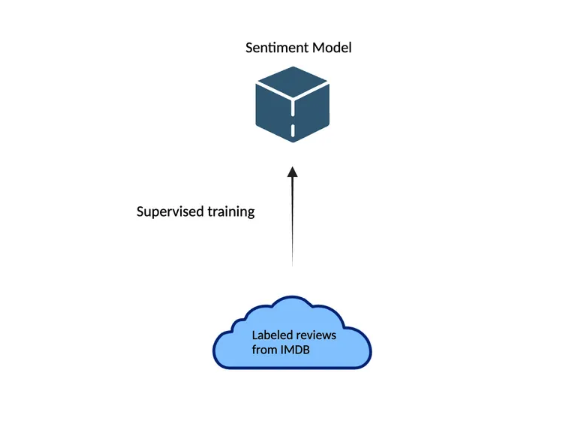
Nowadays, we take advantage of transfer learning:

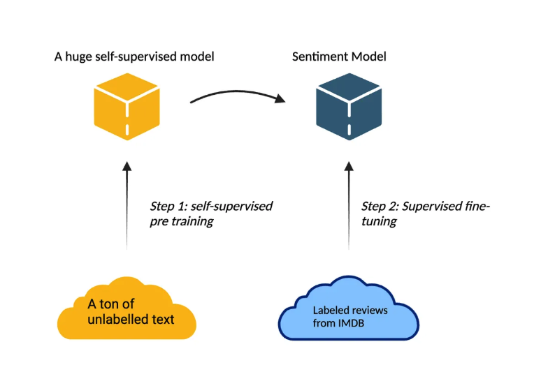
For n-gram models discussion, we focus on language modeling which form the core of Step 1: self-supervised pretraining.

Language Models Assign a Probability to a Piece of Text

---

• Translation: Picking the most likely translation from a list of candidates.
  • P(i flew to the movies) «« P(i went to the movies)
• Speech Recognition:
  • P(i saw a van) »» P(eyes awe of an)

Language models allow us to assign this probability to the words. Example: in search bars.

Probabilistic Language Modeling

---

• Goal: Compute the probability of a sentence or sequence of words.

The Chain Rule

Conditional Probability:

\[P(B | A) = \frac{P(A, B)}{P(A)}\]

Rewriting:

\[P(A, B) = P(A) P(B | A)\]

The chain rule in general:

\[P(x_1, x_2, x_3, ..., x_n) = P(x_1) P(x_2 | x_1) P(x_3 | x_1, x_2) ... P(x_n | x_1, ..., x_{n-1})\]

Chain Rule Applied to Compute Joint Probability of Words in a Sentence

\[P(w_1 w_2 \dots w_n) = \prod_{i} P(w_i | w_1 w_2 \dots w_{i-1})\]

Example Calculation:

For the sentence “its water is so transparent”:

\[P(\text{"its water is so transparent"}) = P(\text{its}) \times P(\text{water} | \text{its}) \times P(\text{is} | \text{its water})\] \[\times P(\text{so} | \text{its water is}) \times P(\text{transparent} | \text{its water is so})\]

• Unigram Model: Calculating the probability of “its” without any context. Frequency of its in the given corpus.

Estimating these probabilities:

\[P(\text{the} | \text{its water is so transparent that}) = \frac{Count(\text{its water is so transparent that the})}{Count(\text{its water is so transparent that})}\]

• This suffers from sparsity because the phrase “its water is so transparent that” might occur only a handful of times in the corpus.
• Also, we aren’t sharing information across semantically similar prefixes in this approach. All prefixes are treated independently, which is inefficient.
• Therefore, we use Markov Assumption: It will not consider words beyond a fixed window size (context length).

\[P(\text{the} | \text{its water is so transparent that}) \approx P(\text{the} | \text{transparent that})\]

• Checkout infini-gram paper.

One Hot Vectors

---

• N-gram models rely on the “bag-of-words” assumption.
• Represent each word/n-gram as a vector of zeros with a single 1 identifying its index.

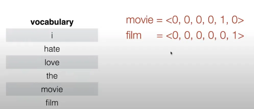
• All words are equally similar, even though “movies” and “film” are semantically similar. There is no information sharing between different words. All words are orthogonal.
• We ideally want a representation space in which words, phrases, sentences, etc. that are semantically similar have similar representations.

Notion of Perplexity

---

• Lower perplexity = better model.
• Perplexity is the exponentiated token-level negative log-likelihood.
• Given a prefix, how many next words are reasonable predictions given that prefix.

\[\text{Perplexity}(\mathcal{W}) = e^{ - \frac{1}{N} \sum_{i=1}^{N} \log P(w_i | w_1, w_2, ..., w_{i-1}) }\]

N-gram Order	Unigram	Bigram	Trigram
Perplexity	962	170	109

Neural Language Models

---

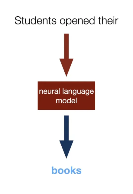
Words as Basic Building Blocks

---

• Represent words with low-dimensional vectors called embeddings.

• There is a loss of interpretation with these numbers. [Research field of explainability]
• The word embeddings start completely randomly.
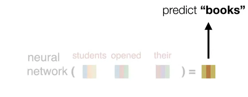
• Neural networks compose word embeddings into vectors for phrases, sentences, and documents. It uses word embeddings to find representations for phrases and sentences.

• Predict the next word from composed prefix representation.

Linear Layer (Feedforward Layer) on the Prefix Vector Representation

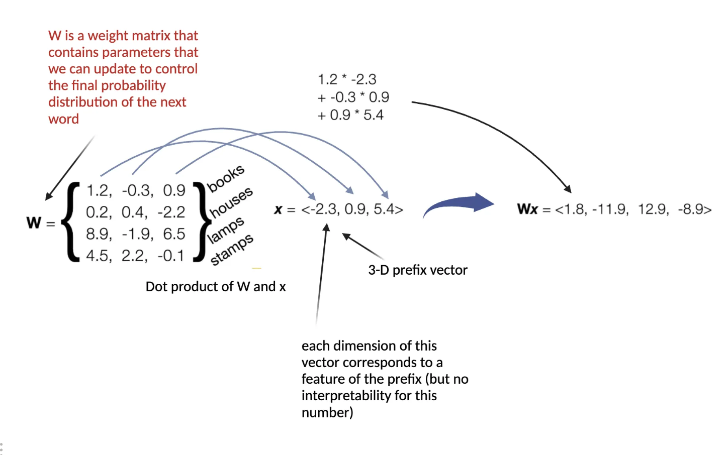
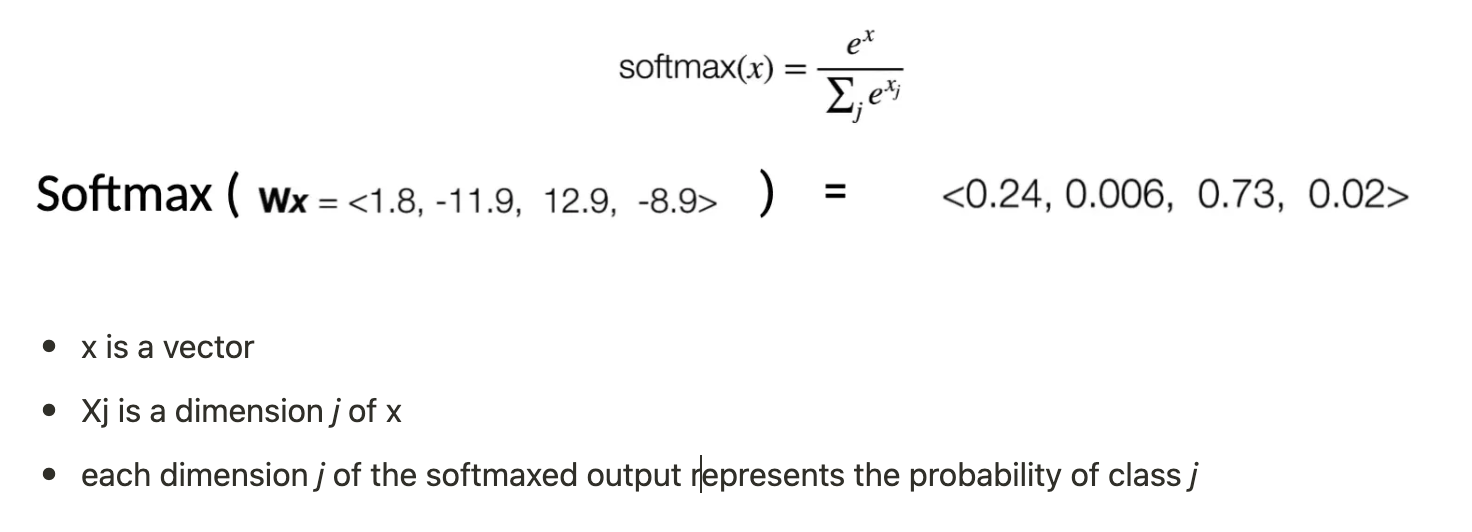
How to go from vector representation (Wx) to a probability distribution of the next word?

• Softmax Layer: Converts a vector representation into a probability distribution over the entire vocabulary.

Different Types of Composition Functions

---

Input: sequence of word embeddings corresponding to the tokens of a given prefix.

Output: single vector.

• Element-wise functions (e.g., just sum up all the embeddings)
• Concatenation
• Feed-forward neural networks
• RNNs
• Transformers

A Fixed Window Neural Language Model

---

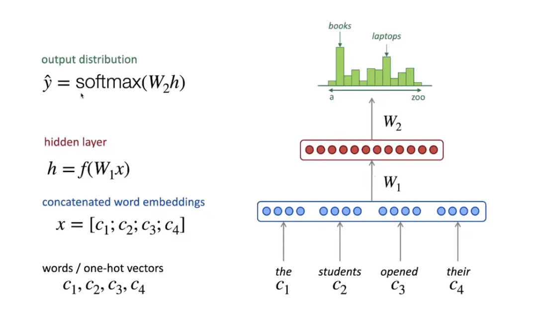
• ReLU non-linearity = max(0, x). Others include tanh and sigmoid.
• f in the above figure is a non-linear function. We want to model non-linear relationships, and therefore there is a need for non-linear functions.

How Does This Compare to Normal N-gram Model?

---

Improvements:

• No sparsity problem.
• Model size is O(n), not O(exp(n)).

Remaining Problems:

• Fixed window size is very small.
• Enlarging window size enlarges W.
• Window can never be large enough!
• Each Ci uses different rows of W. We don’t share weights across the window.

These remaining problems are addressed by Recurrent Neural Networks.

Recurrent Neural Networks

---

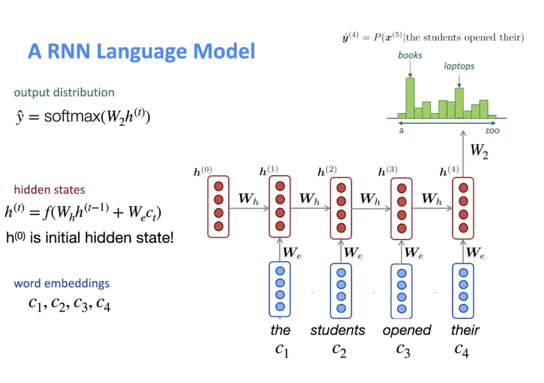
It is sequential and does the calculation from left to right [words of prefix].

• It addresses the problem of not sharing the weights across the window.
• It also takes care of the Markov assumption. Theoretically, there is no limit to t in the RNN equation. We can keep on calculating h(t).

RNN Advantages:

• Can process any length input.
• Model size doesn’t increase for longer input.
• No limit on the size of the window (theoretically). Can use information from many steps back.
• Weights are shared across timestamps → representations are shared.

RNN Disadvantages:

• Recurrent computation is slow.
• In practice, difficult to access information from many steps back.

Neural Language Models [Backpropagation]

---

Training Neural Language Models

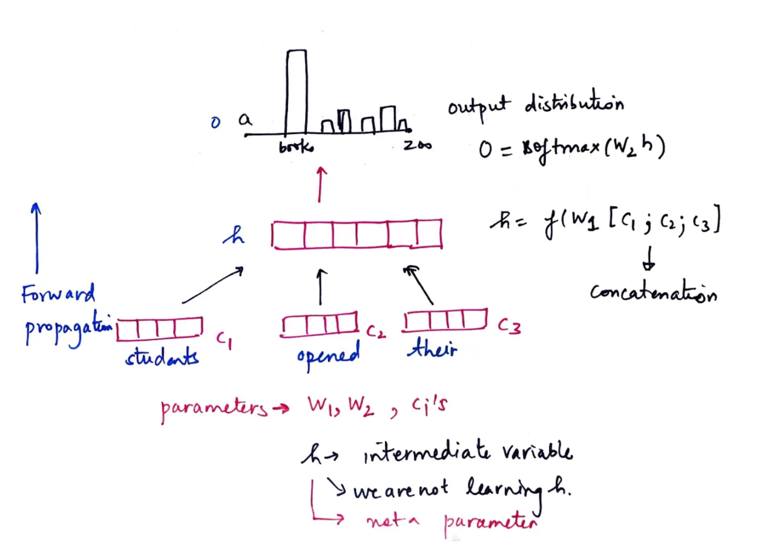
• Last time we talked about forward propagation.
• How can we make NLMs make good predictions?
• NLMs contain parameters (e.g., W1, W2, c1, c2…)
  • These parameters are randomly initialized.

  • Thus, $P(w_1 w_2 \dots w_n) = \prod_{i} P(w_i

    w_1 w_2 \dots w_{i-1})$ is also randomized initially.

• By training the NLM, we adjust its parameters to maximize the likelihood of the training data.

Recap of Forward Propagation

Steps to Train a Neural Language Model

1. Define a loss function L(ϴ), where ϴ refers to all the parameters of the model.
   • This tells us how bad the model is at predicting the next word.
   • Loss function is required to be smooth and differentiable.
2. Given the loss function L(ϴ), we compute the gradient of L with respect to ϴ.
   • The gradient provides us the direction of steepest ascent of the loss function.
   • Step in negative gradient will minimize the loss function. That’s the goal!
   • Gradient is same dimensionality as ϴ.
3. Given the gradient dL/dϴ, we take a step in the direction of the negative gradient.

\[\theta_{\text{new}} = \theta_{\text{old}} - \eta \cdot \nabla_{\theta} L\]

Where:

• $\theta$ represents the model parameters
• $\eta$ is the learning rate
• $\nabla_{\theta} L$ is the gradient of the loss function with respect to $\theta$

Optimizers:

• Gradient Descent parameter: The one shown above is SGD (stochastic gradient descent).
• Other optimizers include Adam, Sophia (LLMs).

Hyperparameters of Gradient Descent:

• Learning rate
• Batch size

Loss Function:

• Loss function: Cross-entropy loss, negative log-likelihood of the next word from the training data given the prefix.